This tipsheet is specific to Microsoft Excel (2007 and newer) for Windows, however other spreadsheet software - such as Google Sheets - have the same functionality. Of course, the buttons and specific ways to do things might be different. But I often find answers by doing a web search using the Excel terms (i.e. how to format cells in Google Sheets). Excel for Mac has all the same functions, but looks slightly different, especially in terms of where buttons and various tools are stored.
Looking around Excel
This tutorial uses a spreadsheet called MLBPayrolls
First, a few things about spreadsheets: Each sheet is made up of columns (labeled by letters) and rows (labeled by numbers). Each cell is identified by a cell address, consisting of the letter and number. For example, in this picture, the value Atlanta Braves is stored in cell A3. Note that when the cursor is on a cell, the cell is outlined in black. Note the small black square in the corner -- we'll be using that in a couple minutes. Also note that the letter and number are highlighted in grey and the cell address is displayed in the upper left corner of the sheet. If you've ever played the board game "Battleship," you'll find this similar.
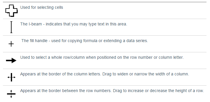
You'll also notice that your cursor will change as you move it around. Most of the time, it will look like a big fat white plus sign. But if you hover over the top of the black box (around Atlanta Braves) you will get a tool that allows you to move that cell and if you hover in the lower right corner - where that little black square is - you will get a thin black cross. That thin black cross is used for copying formulas down or across the page. We'll be using that a lot.
Key terms
- Columns contain "categories" of data and are vertical
- Rows contain invidivdual records and are horizontal
- A cell address consists of a letter followed by a number, i.e. "B4"
- Each Excel file is described as a workbook which can contain multiple worksheets
- The formula bar, which is located in the menu bar, is similar to the address bar in a web browser. Here you can view and edit formulas that you've created in the worksheet.
Cursors
Prepping your data
- Make sure the columns are labeled and that the column label only takes up one row.
- Any notes or titles --or anything else that might be above or below the data table -- should be separated from the data by a blank row (or more). Your data won't sort correctly if other information butts up against the table.
- No empty rows or empty columns within the area where the data is located.
Sorting
There are several ways to change the order that the rows appear in. I'm purposely NOT going to show you the shortcut methods because they don't give you the full suite of options for sorting.
First thing to note: Sorting won't work correctly if you don't have your data set up properly, following the guidelines I noted in the previous section.
Second: Put your cursor somewhere in the chunk of data. Doesn't matter exactly where. Key thing is you don't want it parked out in the whitespace.
Third: Go to the data menu. Click the big button labeled "Sort". This will bring up a dialogue box. Look to see if the checkbox "My data has headers" is checked. If it's not, this is usually a sign that your data is not set up properly. Once that's checked, then the pull-down menu on the left will list the column labels in your data. Select the column label you want to sort on -- in the example, I've chosen Payroll2016 -- and then you can select the order, either Smallest to Largest (ascending) or Largest to smallest (descending).
Note that if you choose the TEAM field, those options will be A to Z and Z to A. That's because TEAM consists of "characters". The Payroll2016 field consists of numbers only (numeric field).
Prep for analysis
The first thing to do is to make sure you understand what you're looking at.
What does each row represent? In this case, it's one row for each team, showing the total they spent on payroll in various years.
Are there any columns you don't understand? This data is pretty straightforward, showing that we have payroll totals for various years (but note that the years are not consecutive). Sometimes, though, you'll get data with a field that has codes in it or something that you don't understand. Be sure to go back to the place you got the data and get your questions answered.
Do you have all the data you need? In this case, the obvious questions might be to ensure you have all the teams you want and that you have payroll totals for all the years you want.
Is there anything missing that would be useful for our analysis? For example, I might want to add a column that indicates which league (AL or NL) each team plays in. It's quite common to need to add something to your data to make it more valuable. (We're not going to do that here, though)
Then you want to come up with the questions you want to ask. We're going into an "interview," so it's a good idea to have a list of questions at the ready. But just like an interview with a human, it's okay to veer off your list at some point later. It helps, though, to have something to start with.
If you're having a hard time coming up with questions, start thinking of the 5 W's -- who, what, when, where, why. Data is really bad at answering the "why" questions, but the others are easier. With this data, our "who" are the teams. We've also got "when" since we have different points in time. The more detailed your data is, the more questions you will be able to ask. This dataset is very limited.
How do I.....?
There are two primary ways to do analysis in Excel. One is by creating new columns or rows to store the results of any formulas you run -- such as creating a new column with percent change or creating a new row with a grand total that combines all the rows. The other is to use PivotTables to generate summaries, either counting rows or summing values together. We'll save PivotTables for the next tutorial (however, I'll note here that it's my favorite tool in Excel).
There are oodles of ways to use formulas and built-in Excel functions to do math, re-arrange your data, clean your data, or even generate new columns to add to your data table. I'm going to focus on a few formulas and built-in math functions that are very commonly used -- percent change, percent of total, average and median.
How formulas work
A formula performs calculations or other actions on the data. It always starts with an equal sign (=), but after that there's a wide array of things you can do, including math calculations and using built-in Excel functions. You type a formula either in a blank column to the right of your data, or in a blank row below your data. And you refer to the cell addresses, instead of the actual values. This allows you to type a math formula one time, then copy the formula and apply it to all the rows or columns of data. As a result, you can do something like calculate percent change for thousands of rows of data in a few seconds. Can you imagine trying to do that on a calculator?
In the video below, I'm going to create two new columns on my table where I'm going to use math formulas to calculate the dollar difference for each department's annual budget figures and then express those differences as percent change. I'll also add some new rows below my data, but I'm keeping it separate with a blank row because these are totals that I don't want mixed into my data table the next time I use sort. I'll cover specifically how to do these formulas and functions later in the tutorial.
Note that I start each with an equal sign, then when I'm finished typing I hit enter. Now my cursor is on the row below. So I need to put my cursor back on the cell where I did the formula, and get the "black thin cross" cursor to copy down my formula to the other rows (or in a couple cases, I copy across columns). You'll notice that you can either drag the thin cross, or you can double-click on your mouse and it will go down until it hits a blank cell in the column immediately to the left. As you copy down, Excel guesses that you want the formula to switch to the next row number. As you copy across, it knows that you want to stay on the same row, but switch to a new column letter.
Percent change
One of the questions you likely came up with for our data is: Which team had the greatest increase (or decrease) in total payroll? So then the next step is to figure out which "tool" in Excel will get us that answer. Here's where you actually need to know a little bit about best practices in math and statistics first.
Let's focus in on two teams, the New York Yankees and the Oakland Athletics. The Yankees paid out more than $222 million in 2016; the Athletics paid out just over $86 million. If we calculate a simple difference between the 2016 and 2011, both teams show that they spent about $20 million more in 2016 than they did in 2011. However, think about these like you would a city budget. A $20 million increase is a drop in the bucket for a city that routinely spends $200 million, while it's a huge increase for the city that spends $60 or $80 million, right?
General rule of thumb is that you'll want to use percent change (rather than simple subtraction) in any situation where the things you are comparing (city budgets, county populations, city crime totals, state spending, school enrollments) have a lot of underlying variability like we have here.
So, let's go back to our full dataset and create a new column to calculate percent change between our two most recent years. I'll add a column label in the first empty column.
The best way to remember the percent change formula is that it's NEW NUMBER minus OLD NUMBER divided by OLD NUMBER. A shorthand way to remember it is the word NO --- (N-O)/O.
This will give you a positive number if it's an increase and a negative number if it's a decrease. Note in the video that after I typed the formula, I ended up with a value expressed in dollars. So I use the format cells option to change it to percentage.
SUM function
This data is a good example of a situation where we might want a grand total -- the total spent on payroll across the whole baseball league. The data didn't come with a total, but even if it did, I'd recommend calculating your own total just to check their work. (I've seen front page stories where news organizations discovered errors in city government totals).
When you have a big column of numbers, the easiest way to get a grand total for a column (or a row) is to use the SUM function. The SUM function requires that you give it a "range" where the data is located. In this case, our data for the first year is stored in cells B3 through B32. The next year of data is C3 to C32, etc. I'm going to add a blank row at row 34, and in cel B34 we'll type our formula: =SUM(b3:b32). Then you can copy that across to the other columns and Excel will automatically adjust the formula, assuming you want to switch to C3:C32 and D3:d32, etc.
Percent of total
We might also want to know what percent of all money spent across the league is made up by the Yankees' monstrous payroll. To do that, we'd calculate percent of total. It will work best if we generate that calculation for all the teams so that we can see how they all compare to each other. In other words, how big is each slice of the pie?
The math for percent of total is to take the team amount and divide by a total for the whole league. It's a good thing, then, that we just calculated those totals in the step above. For this one, we'll just calculate the percent of total for the most recent year and we'll put that in the first blank column to the right of our data. Our formula will be the first team's value for 2016 -- located in cell I3 -- divided by the league total -- located in cell I34. However, if we run that it works for the first row but we get an error message on the subsequent rows. If you look at the formula for the second row, you can see the problem. Excel guessed that you wanted to change the formula to I4/I35. You can see that I4 is correct, but what's in I35? Nothing.
So we need to tell Excel to ALWAYS stay on I35. This is called an anchor. Excel uses a dollar sign ($) as an anchor. If you put a dollar sign in front of the letter in the cell address, it will always stay on the I column, but the row number could adjust automatically. If you put a dollar sign in front of the number in the cell address, it will stay on the row, but could adjust column letter if you copy across. Or you can put dollar signs in both positions to lock on that one cell. That's what we'll do here. (And yes, there are situations where you only want to anchor one but not the other.)
So go back to the original formula in I3 and adjust the formula -- =I3/$I$34 and then copy that down.
AVERAGE and MEDIAN functions
Just like how we totaled a column of numbers using the SUM function, we can also calculate the average or the median for a given column, using the AVERAGE and MEDIAN functions that are built into Excel. It works the same way: =AVERAGE(B3:B32) or =MEDIAN(B3:b32)
The rule of thumb in using average versus median is that you should use median (which returns the middle value) in situations where you have big outliers -- either a few values that are really low or really high compared to the majority of the other values. This happens a lot with salary records or home sale prices, for example. You can test whether a median is warranted by calculating both on your dataset. If the two numbers are close together, you'll be okay using average. If they are not, then use the median.
Shortcuts and other useful tricks
To highlight your block of data, put your cursor somewhere in the middle of your data, then push control-shift-asterisk (*) at the same time. (Only works in Windows)
To check the four corners of your highlighted data chunk, highlight your data (using the trick we just mentioned), then push control-period (.) at the same time. And repeat this four times. Each time you push the keys, it will go to a different corner of the data. This is useful for mkaing sure you have highlighted the full chunk (and nothing extraneous) before sorting or copying.
Freeze panes is a useful way to keep your headers at the top of the page, so you can see them when you scroll down a big dataset. Place your cursor in the cell just below the row you want to lock into place (usually this would be somewhere around A2 or A3, depending which row your data starts on). Then go to the View menu and select "Freeze panes." It will give you several options, such as freezing the top row or freezing one or more columns on the left, plus the top row.
To return to the top of your data push control and home keys at the same time. It will take you to A1.
To highlight an entire column put your cursor on the first cell of data, then push control-shift and the down arrow key. It will highlight all the way down until it hits a blank row. It works the same for rows, except you would push control-shift and the right arrow key.
Paste Special allows you to get rid of formulas, so that only the answers remain. Think carefully about whether you want to do this, though. Sometimes leaving the formulas there gives you a sort of "paper trail" of what you did, or allows others to see what you did. To use Paste Special, highlight the row(s) or column(s) that have the formulas. Copy the data using Ctrl-C or the copy button. Then put your cursor where you want to paste the data and right-mouse click, then choose "Paste Special." A little box will come up: Under the Psate section at the top, choose "Values" and push OK.
Hide columns: You can hide columns to get them out of your way or to avoid printing them by highlighting the columns you want (click on teh letter at the top of the column) and right-mouse click to choose "Hide columns." The columns will disappear. To get them back, highlight the two columns on either side of the ones that are missing and right-mouse click and choose "Unhide columns."
Add columns or rows: To add a new column in the middle of your data, click on the letter of the column immediately to the RIGHT of where you want the new column. Make sure the whole column is highlighted (if you click on the letter above the column Excel will automatically highlight the whole column). Then right-mouse click and choose "insert." To add a new row, click on the number of the row just BELOW where you want the new one. Make sure the whole row is highlighted, then right-mouse click and choose "insert."
Worksheets: You can toggle between different worksheets in an Excel workbook using the tabs in the lower-left corner. They have default names of "Sheet 1" or "Sheet 2", etc. To change the name, double-chick on it and it will turn black-- then you can start typing a new name. To add a new worksheet, you'll see a little button to the right of the tabs to add a worksheet. You can move worksheets around so they appear in a different order.
That's it for this tutorial. Thanks for making it to the end! You can find more advanced Excel tutorials on my main training page.